1.4 Data analysis and decision making
Participants: J. Arnó, J. Llorens, J.A. Martínez-Casasnovas, J.R. Rosell-Polo, A. Escolà, L. Sandonís.
Geostatistics and spatiotemporal data analysis
The use of proximal and remote sensors in Precision Agriculture allows different types of data on crops and / or the environment in which they are grown to be acquired. In general, data spatial resolution is usually high if a yield sensor is used acquiring data continuously (on-the-go), or is rather low (few data per hectare) when data is acquired manually and in a discreet manner (for example, counting the number of grape clusters per vine). In any case, mapping data is considered a fundamental previous step to facilitate the analysis and the interpretation of information.
Current practice of Precision Agriculture makes it advisable to obtain surface maps (maps with raster coverage), for which the use of spatial interpolation techniques is essential (Figure 1). Among the different existing possibilities, geostatistics allows, apart from mapping the data, indication of the present uncertainty or error in maps to be obtained. In a simplified way, obtaining maps using geostatistical techniques includes two differentiated steps, i) variographic analysis, where the spatial variation structure (semivariogram) of the variable to be mapped is assessed and, ii) geostatistical interpolation (kriging) which, based on the semivariogram, it makes possible the prediction of the variable in unknown points or pixels (grid points) that cover the geographic area to be mapped. There are different computer programs for geostatistical interpolation. The VESPER program (https://precision-agriculture.sydney.edu.au/resources/software/download-vesper/) is an interesting and recommended option by our research group. Some notable features of the program are the performance of point or block interpolations, and the possible use of local variograms when the assumption of quasi-stationarity is assumed (that is, when a large number of data is available on an area of some or great extent).
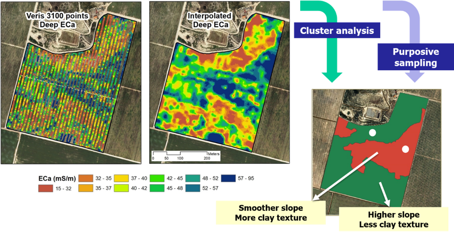
Figure 1. Map of apparent electrical conductivity (CEa) (central map) after applying a geostatistical interpolation to the initial data provided by a soil sensor (map on the left). The classification of the interpolated map (cluster analysis) has made it possible to segment two soil classes for differentiated irrigation management at the plot level. Finally, optimal location of humidity probes for irrigation monitoring in each of the classes has been established based on purposive sampling.
On-farm experimentation
On-farm experimentation refers to the assessment of different management techniques that are implemented on commercial farms by the farmers themselves. Unlike 'conventional' experimentation, carrying out 'on-farm' experiences prioritizes the interest of the farmer and makes use of the data from his farm to optimize the production processes normally used in the area. Under proper advice, carrying out this type of experimentation is a practical way to make known and spread the adoption of Precision Agriculture technologies. On the other hand, experimentation is usually carried out on a wide spatial scale (plot or farm), which allows capturing an important part of the space-time variability that occurs at the farm level.
Our research group has launched several on-farm experimentation projects. For example, Figure 2 shows the plot where an evaluation test of the efficacy of a bioactive compound for the control of water stress in corn has been carried out. Having delimited different dosage sectors, this experimentation has allowed all the agents involved to be benefited. The farmer has found a possible solution to a relevant problem in his farm. The supplier company has been able to demonstrate the reliability and conditions of use of the product it offers. Regarding the GRAP, the researchers of the group have been able to apply statistical methods of space-time analysis on satellite images, and thus adequately interpret the effect of the different irrigation management strategies that had been proposed
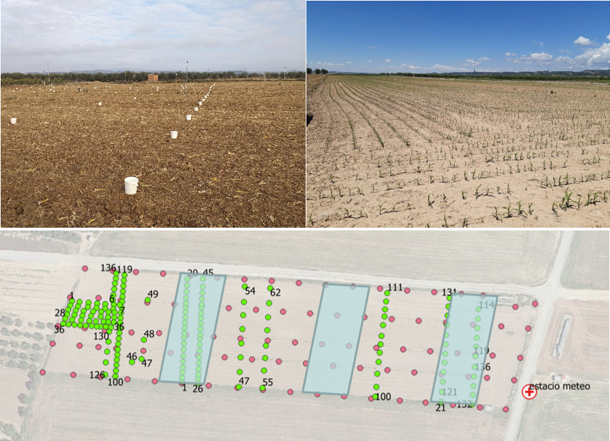
Figure 2. ‘On-farm’ experimentation on irrigation management and water stress in maize.
Site-specific management and variable rate technologies
Through on-farm experimentation, our group (GRAP) has been able to evaluate the advantages of using different variable rate technologies. Figure 3 shows a real case of differentiated application of fertilizers in an extensive plot. Based on the map of the apparent electrical conductivity (CEa) of the soil (map A) and the vigour map (NDVI, Normalized Difference Vegetation Index, map B) of the preceding maize crop, a fertilization prescription map is proposed (map C) differentiating three doses according to the characteristics of each zone. The final gross economic margin map (map E) derives from subtracting from the harvest map (map D), multiplied by the sale price of the grain, the cost of differentiated fertilization in each area (map C). Despite the fact that the final objective is to equal the benefit throughout the parcel (in an attempt to adjust the resources applied to the productive potential of each zone), it is verified that the gross margins are spatially variable. Therefore, it will be necessary to readjust the actions in successive campaigns based on the results and experience gained from the recursive application of fertilizers at variable doses. Often, the benefits of opting for Precision Agriculture and variable application technologies are obtained in the medium and long term, being necessary to learn from several campaigns before increasing the profit of the farm due to better management of the resources used.
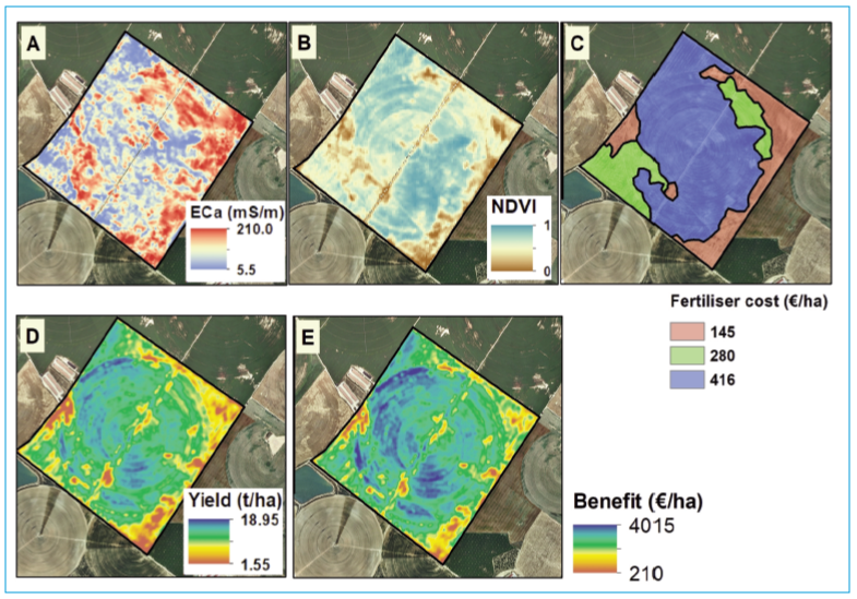
Figure 3. Differentiated management of fertilization in a 100 ha extensive farming plot. A: map of apparent electrical conductivity (CEa); B: NDVI map of the previous maize crop; C: fertilization prescription map; D: yield map resulting from the differentiated application of fertilizers; E: map that indicates the gross margin obtained (€/ha) by subtracting the cost of fertilization from the yield map multiplied by the sale price of corn.